Rejection Number
Meaning ~ The rejection number is the minimum count of defective units in a sample that triggers the formal rejection of a production batch under a sampling plan.

Threshold
The rejection number is the minimum count of nonconforming units in a random sample that legally and statistically triggers the rejection of an entire production lot under an attribute sampling plan. In quality assurance, this number marks the boundary where a batch stops being an asset and becomes a legal liability. Pulled from standard statistical tables, it is written directly into supply contracts to prevent disputes during pre-shipment inspection.
Setting a clear limit on process variation protects buyers from bad inventory while giving suppliers a predictable tolerance. Once a sample crosses this threshold, the buyer can refuse the shipment, demand full sorting, or enforce contract penalties.
That boundary applies specifically to attribute-based acceptance sampling, where each inspected item passes or fails. If testing measures continuous dimensions on a scale, variables sampling plans calculate the sample mean and standard deviation to estimate total defect rates, making single-defect counts irrelevant. Nor does the metric apply to continuous production runs monitored by real-time process control charts rather than lot-by-lot checks.
High-volume electronics assembly, for instance, often relies on automated scanning and defects-per-million calculations instead of conventional sampling tables. The rejection number belongs to lot-by-lot attribute audits, where sample results decide whether an entire shipment moves forward.
Statistical Boundaries of Lot Quality
Friction in overseas manufacturing usually comes down to the gap between a batch’s true defect rate and what an inspector finds in a sample. No sampling plan guarantees a flawless production run, so the rejection number acts as a statistical filter to manage risk for both parties. Setting this threshold establishes the plan’s operating characteristic curve, plotting acceptance probabilities across actual defect rates.
Buyers and suppliers negotiate these limits to establish clear contractual ground rules. When a sample hits the rejection limit, the likelihood that the whole batch exceeds agreed defect tolerances is high enough to justify rejecting it.
The decision itself is strictly binary, which keeps debate off the factory floor. If an inspector finds fewer defects than the rejection threshold, the lot passes, even if the sample contains flawed units. That reflects the reality of mass production, where minor variation is inevitable.
Removing subjective judgment holds both parties to the agreed standard and translates statistical probability into a pass-or-fail outcome.

Attributes and Variables Inspection
Choice of sampling method depends on product type and testing cost. Attribute sampling ~ which relies on rejection numbers ~ is standard for visual checks, assembly verification, and quick non-destructive tests. Each unit is classified as conforming or nonconforming against clear criteria.
Variables inspection measures specific physical traits like torque, weight, or tensile strength, yielding equivalent statistical confidence from smaller samples, though it requires calibrated equipment and detailed record-keeping. Attribute sampling dominates consumer goods, textiles, and molded plastics because it is straightforward to run and simple to execute on the shop floor.
When a lot fails, the justification rests entirely on the sampling plan specified in the contract. Importers protect their margins by stopping shipments the moment defect counts cross that clear boundary.
Standard
Acceptance sampling relies on published international tables to convert lot sizes and risk tolerances into specific testing numbers. The main references in international trade are ISO 2859-1 and ANSI/ASQ Z1.4, both derived from the military standard MIL-STD-105E. These standards link batch sizes directly to sample sizes and pass-reject criteria so that an inspection on a workbench in Ningbo yields results statistically consistent with an audit at a warehouse in Rotterdam.
Using the tables involves a two-step lookup. First, the inspector matches the total batch size ~ the lot size ~ against the chosen inspection level to find a letter code between A and R. General Inspection Level II is the standard baseline for most goods, balancing inspection effort against risk. Level I reduces sample sizes for proven suppliers, while Level III increases sample sizes for added protection with unverified factories.
That letter leads to the master table, which gives the exact sample size alongside acceptance and rejection limits for the target quality levels.
The Structure of Attribute Sampling
In a single sampling plan, acceptance and rejection numbers sit back-to-back: the rejection threshold is always exactly one defect higher than the acceptance limit. If the table sets the acceptance number at five, six defects trigger a rejection. An inspector cannot make an exception for a six-defect sample, regardless of the factory’s explanation or the shipping schedule.
That strict separation is built into attribute standards specifically to head off disputes and enforce objective decisions.
Standard tables derive from binomial and hypergeometric distributions that calculate the probability of pulling defective units from a lot at various defect rates. The plans are organized around the Acceptance Quality Limit (AQL), which defines the highest average defect rate tolerated over time. Limits typically range from 0.065% for critical components to 4.0% for minor cosmetic flaws in consumer products.
Matching the sample code letter with the target AQL gives the inspector the required sample size and the exact rejection number for that lot.

Inspection Levels and Sample Code Letters
To show how these rules work in practice, the table below outlines sampling plans generated under ISO 2859-1 for Normal Inspection Level II across typical batch sizes and quality limits, showing how sample sizes and rejection numbers scale with lot volume.
| Lot Size (Units) | Code Letter | Sample Size (n) | AQL 1.0% (Ac / Re) | AQL 2.5% (Ac / Re) | AQL 4.0% (Ac / Re) |
|---|---|---|---|---|---|
| 151 to 280 | G | 32 | 0 / 1 | 2 / 3 | 3 / 4 |
| 281 to 500 | H | 50 | 1 / 2 | 3 / 4 | 5 / 6 |
| 501 to 1,200 | J | 80 | 2 / 3 | 5 / 6 | 7 / 8 |
| 1,201 to 3,200 | K | 125 | 3 / 4 | 7 / 8 | 10 / 11 |
| 3,201 to 10,000 | L | 200 | 5 / 6 | 10 / 11 | 14 / 15 |
| 10,001 to 35,000 | M | 315 | 7 / 8 | 14 / 15 | 21 / 22 |
| Methods note: Derived from ISO 2859-1 single sampling plans for normal inspection. Ac represents the acceptance number, and Re represents the rejection number. Arrows in original tables dictate using alternative plans if the intersection does not yield a specific number. | |||||
A lot consisting of five thousand widgets evaluated under level two parameters requires a sample size of two hundred units.
These figures illustrate the efficiency gains of larger batches. Increasing a lot from five hundred to ten thousand units is a twenty-fold jump in production volume, but the required sample size only moves from fifty to two hundred pieces. That economy of scale is why buyers prefer larger manufacturing runs over frequent small orders: it lowers per-unit inspection costs without compromising statistical protection.
Under ISO 2859-1 Clause 10.3, charges for re-inspecting or storing rejected lots are billed directly to the factory.

Bench
Carrying out a pre-shipment inspection starts by pulling random samples from packed export cartons. Inspectors on the factory floor avoid pulling only from accessible front pallets, using a random number generator to select cases across the top, middle, and bottom of stored pallets for a representative sample. Those units move to a designated workbench with clean surfaces and calibrated equipment so shop conditions do not skew results while nonconforming units are counted.
Inspectors check each unit step by step against the specification sheet, starting with visual finish before checking dimensions and function. Every defect is logged into a distinct severity tier: minor defects cover cosmetic flaws that leave functionality intact, major defects impair performance or durability, and critical defects introduce safety hazards or render the item unusable. Tallies are kept separate for each tier, and a lot fails if any single category reaches or exceeds its rejection limit.

Defect Categorization on the Line
Sorting out defect tiers requires clear contract definitions to avoid disputes on the shop floor. Factory staff often try to reclassify major structural flaws as minor surface issues. Visual defect guides, boundary samples, and reference pieces settle those disagreements.
If a flaw matches the contract description of a major defect, it is logged accordingly. Sourcing teams track these categories separately because each has its own rejection limit; a batch can easily pass its minor defect threshold and still fail over a single critical safety defect.
Field offices stay in close touch with inspectors during audits. Factory personnel watch defect counts closely as work proceeds, and tension rises quickly when major defect counts approach the threshold. That makes accurate defect calls essential.
Inspectors take detailed photos and stream live video of questionable items to make findings indisputable before comparing final tallies against the sampling plan.
Early Termination in Sampling Runs
An inspection can end early if defect counts hit the rejection number before the full sample is examined. If a plan requires pulling two hundred units with a rejection limit of eight, and the inspector finds eight major defects in the first fifty pieces, the batch has already failed. Continuing through the remaining one hundred and fifty items will not alter that statistical outcome.
Stopping the audit saves time and lets the factory begin sorting immediately, provided the final report still gives the buyer a complete picture of the failure.
Here is how these criteria apply in practice. Sourcing managers rely on the rejection threshold to determine whether lots pass or fail during field audits.
- rejection number marks the strict boundary where sample findings halt the movement of a production batch.
- rejection numbers give factory supervisors a concrete target for scheduling rework before the vessel sailing date.
- rejection number‘s breach forces the quality team to issue a formal non-conformance report to purchasing.
- rejection number governs the outcome of a pre-shipment audit by capping allowable sample defects.
While high humidity during production can cause surface defects, passing affected items through an air-dryer rarely restores a nonconforming batch to contract specification.

Contract
Importers use purchase contracts to define the statistical rules governing when ownership shifts from seller to buyer. The applicable standards, inspection levels, and rejection numbers belong directly in the purchase order or master agreement. Without those details in writing, a buyer has little legal standing to reject a shipment with excessive defects.
Sourcing teams avoid vague terms like “high quality” or “commercial grade,” specifying instead the exact standard used, what happens when defect limits are breached, and that title remains with the supplier until inspection passes.
That contractual clarity is vital under international commercial terms. In FOB agreements, title and risk usually pass to the buyer once cargo crosses the ship’s rail at origin. However, if a pre-shipment inspection shows the rejection number has been hit, the buyer can reject the goods before loading.
Sourcing agreements make title transfer contingent on a passing inspection certificate; without it, the supplier retains ownership of the inventory at the factory, and the issuing bank blocks payment.

What Occurs When a Lot Fails Inspection?
A failed audit triggers a defined sequence of contractual steps. The buyer issues an immediate non-conformance report accompanied by defect logs and workbench photos. The supplier then has a set window to submit a corrective action plan showing how nonconforming items will be isolated, scrapped, or replaced.
Buyers rarely permit a factory to resubmit a lot without a documented sorting process, which typically leads to a second failure. Contracts also assign re-inspection fees and extra storage costs directly to the supplier.
This procedure protects buyers from carrying financial losses or absorbing avoidable delays. The steps below trace the standard resolution path after a lot fails on the floor.
- The buyer transmits the purchase order with the specified quality limits to the manufacturer.
- The manufacturer completes the production run and places the finished goods in the export warehouse.
- The inspection agency draws a random sample based on the agreed sampling plan.
- The agency issues a passed or failed inspection certificate based on the defect count.
- The forwarder uses the passed certificate to book ocean carriage and release the letter of credit.
The purchase contract designates that the factory bears all financial liability for shipping delays arising from a failed quality audit.

Risk Allocation and Incoterms Mechanics
Connecting quality inspection to payment mechanisms is critical in overseas trade. Under a letter of credit, the bank releases funds only if the exporter presents compliant shipping documents. Sourcing contracts frequently make a passing inspection certificate mandatory for payment.
If the defect count reaches the rejection limit, no certificate is issued and the bank will not honor the draft, preventing payment for sub-standard goods.
That leaves open the question of whether a buyer can claim damages for missed retail sales when a rejection occurs too close to a key holiday deadline to allow for re-production.
Arithmetic
Evaluating the financial cost of statistical error helps quality managers balance factory exposure against buyer risk. Sourcing teams use operating characteristic curves ~ which chart acceptance probabilities against actual defect percentages ~ to measure how much protection a plan offers. The two primary metrics are producer’s risk (the odds of rejecting an acceptable batch) and consumer’s risk (the odds of accepting a lot that exceeds defect limits).
Calculating these risks relies on the binomial distribution. In a single sampling plan with a sample size of two hundred pieces, an acceptance number of seven, and a rejection threshold of eight, a lot with a true defect rate of 1.5% has an acceptance probability of roughly 98% ~ leaving a producer’s risk of just 2%. Sourcing teams favor this arrangement because a well-made batch consistently passes inspection.

Operating Characteristic Curves and Risk
If factory process control slips and the defect rate jumps to 5%, the risk profile shifts completely. The chance of finding seven or fewer defects in that two-hundred-unit sample drops to around 22% ~ meaning there is a 22% consumer risk that a 5% defective lot will pass and ship out. For sensitive applications like automotive parts or medical devices, a 22% chance of accepting bad stock is unacceptably high.
Buyers respond by tightening the AQL or increasing the sample size to push consumer risk down.
Sourcing teams often advise buyers to switch to tightened inspection when working with suppliers that have spotty quality records. Tightened inspection lowers both the acceptance and rejection numbers for a given sample size, making it much harder for borderline batches to slip through. The points below illustrate how setting the rejection threshold shifts risk during an audit.
- rejection number marks the point where sorting costs fall entirely on the manufacturer.
- rejection numbers directly determine consumer risk calculations on operating characteristic curves.
- rejection number prevents suppliers from slipping marginal product into larger export shipments.
- rejection number triggers contractual remedies if a supplier fails to rework defective items.
Sourcing teams frequently accept a minor defect threshold breach in exchange for a retroactive purchase price adjustment.
Producer and Consumer Risk Analysis
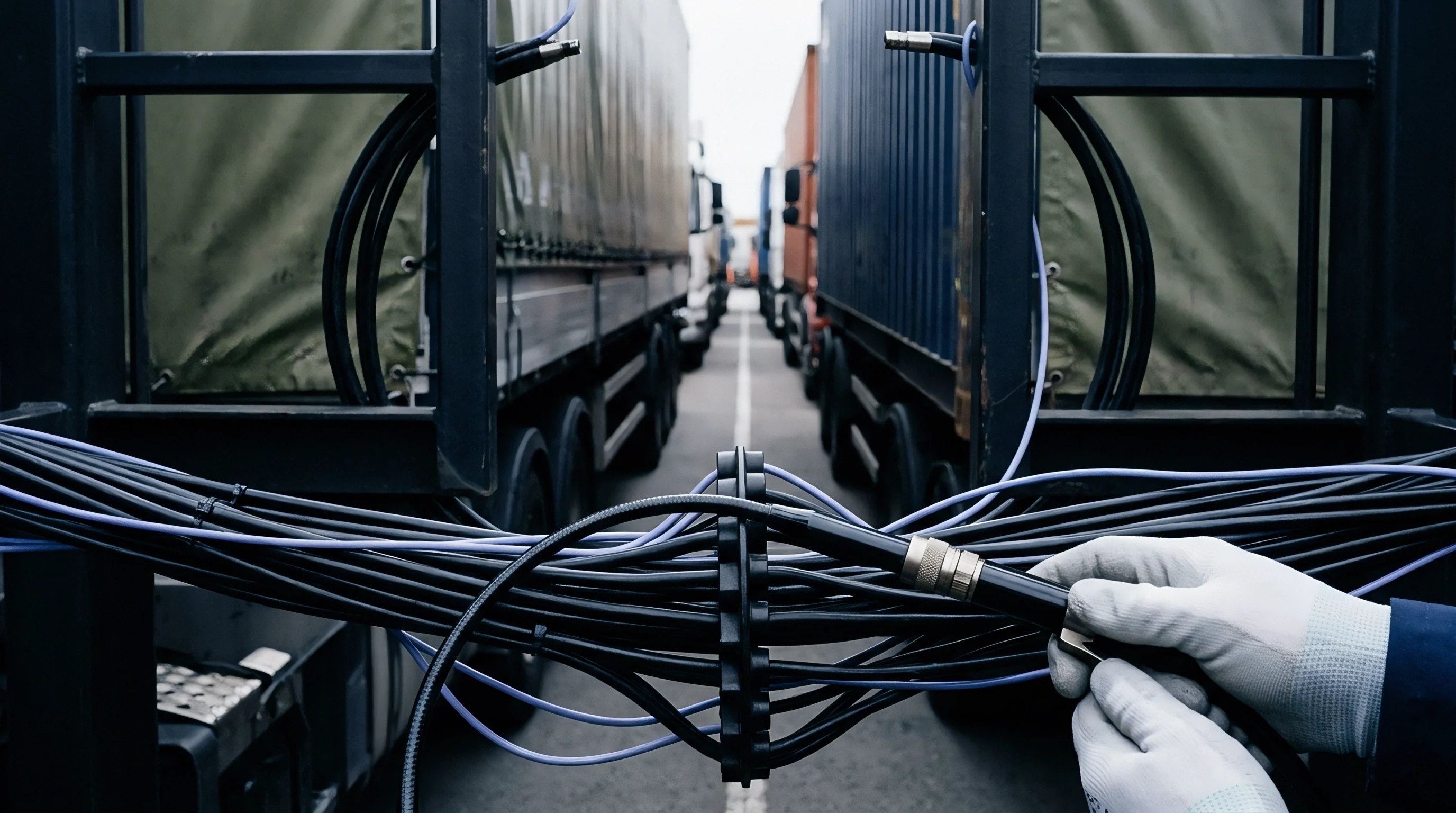
Consider a concrete example: an order of ten thousand custom high-voltage cable harnesses priced at ten dollars each. Under General Inspection Level II, the sample size is two hundred units. With an AQL of 1.5% for major defects, the acceptance number is seven and the rejection threshold is eight.
If the auditor logs nine defects, the lot fails, leaving the factory with two thousand five hundred dollars in labor to unpack, sort, and repack all ten thousand units, plus an eight hundred dollar re-inspection fee.
Importers sometimes incur charges ~ such as four thousand dollars to fly a regional lead auditor from Singapore to Ho Chi Minh City ~ to re-inspect a rejected lot of circuit boards after a supplier challenges local laboratory calibration records.

Dock
A failed inspection causes immediate operational disruptions at both the factory and the port. When a lot is rejected on the floor, loading stops and disrupts the shipping timeline. The export coordinator must cancel container bookings and reschedule the vessel, which often brings late cancellation fees and extra drayage costs if the container is already en route.
Missed sailings can push destination warehouse delivery back by several weeks while rework takes place.
The factory must also isolate rejected goods in a secured, clearly marked red-tag quarantine area so they are not mixed into good stock or loaded accidentally. Sourcing teams insist that sorting starts immediately to limit delays. Rework is labor-intensive, requiring workers to unpack every case, inspect every item, and replace defects with passing units at the supplier’s expense.

Logistical Scenarios for Failed Batches
The financial fallout of a failure depends on where it is caught. If detected during pre-shipment inspection at the factory, the supplier pays for rework and re-inspection. If caught after arrival at the destination warehouse, costs balloon as the importer faces return freight, customs duties, and disposal fees ~ a scenario that almost always sparks bitter disputes over refunds or credits.
Pre-shipment audits exist specifically to catch defects before goods leave the factory floor.
Factories cooperate quickly when a rejection is backed by clear data. The table below outlines how costs and operational responsibilities break down depending on when a failure is identified.
| Escalation Stage | Operational Action | Supplier Cost Share | Importer Cost Share | Landed Cost Impact |
|---|---|---|---|---|
| Pre-Shipment Failure | Sorting and Rework | 100% of rework labor and packaging | $800 re-inspection fee | +2% to +5% due to delay |
| Port-Side Failure | Return to Factory | Container drayage and terminal fees | Demurrage after five days | +15% due to shipment delay |
| Destination Warehouse | Total Rejection or Scrap | Cargo value and ocean freight | Retesting and disposal fees | +110% due to line shutdown |
| Summary: Re-inspection fees and logistics are shared or allocated based on contract terms, with late failures resulting in severe landed cost increases and shipment delays. | ||||
Inspectors often confront intense hostility from factory owners when the count of nonconforming units sits on the edge of the rejection limit.

Rework and Scrap Cost Calculations
Whether to rework or scrap a lot comes down to product value versus labor cost. Suppliers almost always sort high-value electronics, where scrapping represents a severe loss. Sorting cheap molded plastic toys, however, can easily cost more in labor than the inventory is worth, leading the factory to scrap the lot and restart production.
Sourcing agencies oversee disposal of scrapped goods to keep defective stock off the grey market.
This statistical and contractual discipline helps keep international supply chains stable. To sourcing managers, the rejection number is more than a formula ~ it protects product quality, brand reputation, and profit margins. A clear numerical benchmark ensures buyer and supplier operate under identical expectations, minimizing friction and keeping trade moving even when factory defects occur.